Part 2 of the 600,000 Questions benchmark series
TL;DR
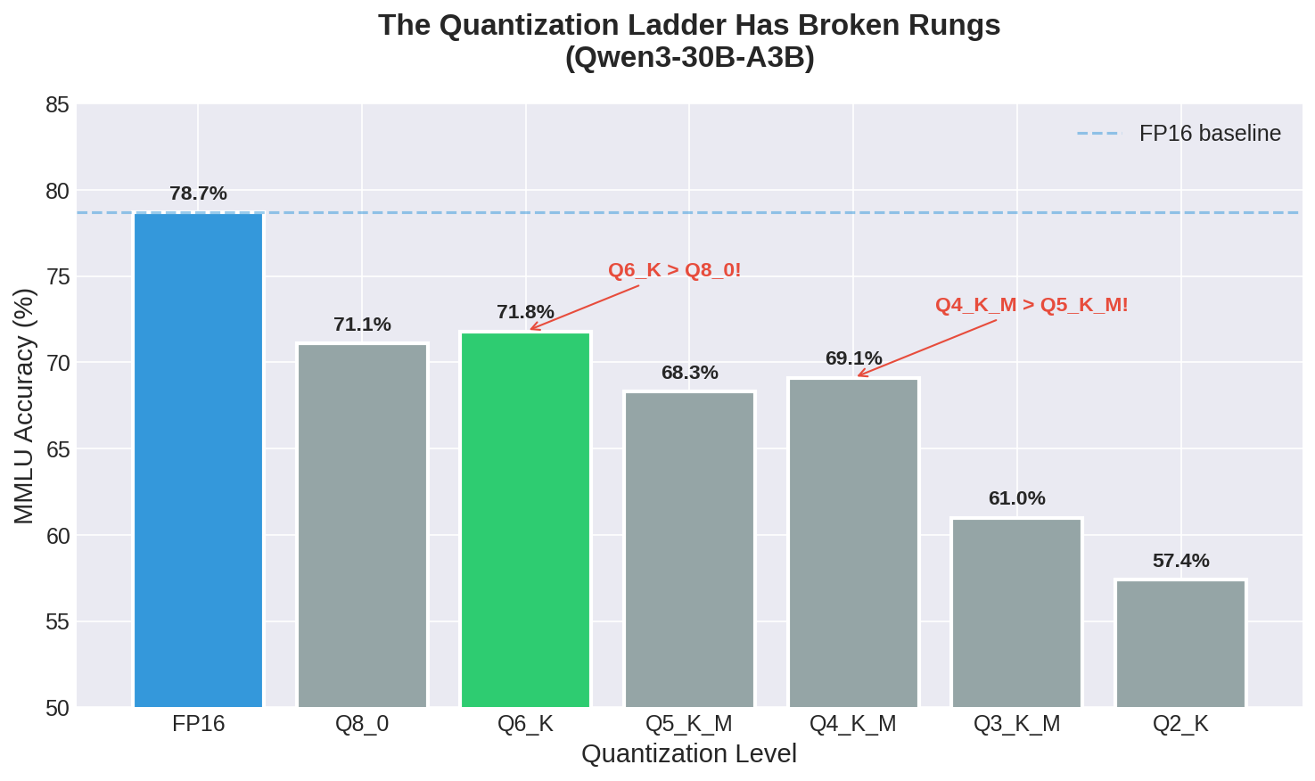
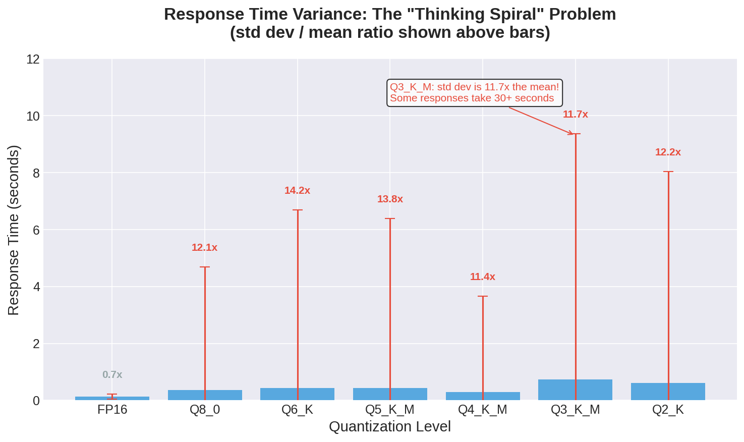
Testing Qwen3-30B-A3B across seven quantization levels revealed that the accuracy-vs-quantization relationship is not monotonic. Q6_K (71.8% MMLU) outperforms Q8_0 (71.1%), and Q4_K_M (69.1%) beats Q5_K_M (68.3%). The explanation lies in how K-quant schemes allocate precision: Q6_K uses smarter mixed-precision than Q8_0’s uniform approach. Response time variance tells an even more dramatic story—quantized models have standard deviations 10-14x their mean response times, indicating unpredictable “thinking spirals” that occasionally run 30+ seconds for simple questions. The practical implication: Q4_K_M offers the best balance of speed (0.294s), memory efficiency, and accuracy (69.1%) for the 30B model class, but FP16 remains superior if you have the VRAM.
Every discussion of model quantization includes some version of the same chart: a smooth curve showing accuracy declining as you reduce precision from FP16 to Q8 to Q4 to Q2. The curve slopes gently at first—”minimal quality loss down to Q4”—then drops off a cliff at the extreme low end. This mental model is so pervasive that I had it internalized before I ever ran a single benchmark.
The actual data from Qwen3-30B-A3B does not follow that smooth curve.
Here’s what I measured across 14,042 MMLU questions for each quantization level:
| Quant | Accuracy | Delta from FP16 | Avg Time | Std Dev | tok/s |
|---|---|---|---|---|---|
| FP16 | 78.7% | baseline | 0.129s | 0.086 | 210.9 |
| Q8_0 | 71.1% | -7.6% | 0.357s | 4.331 | 229.4 |
| Q6_K | 71.8% | -6.9% | 0.440s | 6.249 | 237.2 |
| Q5_K_M | 68.3% | -10.4% | 0.432s | 5.953 | 245.4 |
| Q4_K_M | 69.1% | -9.6% | 0.294s | 3.359 | 252.7 |
| Q3_K_M | 61.0% | -17.7% | 0.736s | 8.630 | 242.3 |
| Q2_K | 57.4% | -21.3% | 0.609s | 7.426 | 249.4 |
Notice anything strange? Q6_K outperforms Q8_0. Q4_K_M outperforms Q5_K_M. The smooth curve isn’t just imperfect—it’s not even monotonic.
Why K-Quants Break the Rules
GGUF quantization isn’t a simple “reduce all weights to N bits” operation. The K-quant schemes—those with _K, _K_M, or _K_S suffixes—use mixed-precision approaches that allocate different bit depths to different parts of the model based on importance analysis.
Q8_0 is a uniform 8-bit quantization. Every weight gets the same treatment. It’s simple, predictable, and was the gold standard before K-quants came along.
Q6_K uses 6-bit quantization for most weights but preserves higher precision for the most important weights identified through sensitivity analysis. The “K” indicates this is a “K-quant” scheme that varies precision across the model.
When the sensitivity analysis correctly identifies which weights matter most, Q6_K can preserve the critical computational paths while aggressively compressing the less important ones. The result is a model that’s smaller than Q8_0 but more accurate on certain tasks, because the important weights that Q6_K preserves in higher precision are more critical than the uniform precision that Q8_0 maintains everywhere.
This explains the Q6_K > Q8_0 result. But what about Q4_K_M > Q5_K_M?
The _M suffix indicates “medium” in the K-quant scheme—a balance between size and quality. Q4_K_M is more aggressively optimized than Q5_K_M, with more research having gone into identifying optimal precision allocation at the 4-bit level. The 5-bit schemes were implemented later and arguably received less tuning. Sometimes the second-best option is better than the theoretically-superior one simply because more engineering effort went into it.
The Variance Problem
Look at the standard deviation column in that table. FP16 has a standard deviation of 0.086 seconds—responses are tightly clustered around the 0.129 second mean. That’s what you want in a production system: predictable latency.
Now look at Q3_K_M: mean of 0.736 seconds, standard deviation of 8.63 seconds. The standard deviation is eleven times the mean. This isn’t a normal distribution with a long tail—this is a bimodal distribution where most questions are answered in under a second but some questions trigger extended reasoning loops that run for 20, 30, even 60+ seconds.
I dug into the detailed logs to understand what was happening. For a question like “What is the capital of France?”, the FP16 model outputs something like:
The capital of France is Paris.

A
The Q3_K_M model occasionally outputs:
Let me think about this step by step.

France is a country in Western Europe. I need to recall its capital city.

Major cities in France include Paris, Lyon, Marseille, and Nice.

The capital of a country is typically its largest city and seat of government.

Paris is the largest city in France and serves as the seat of the French government.

Wait, let me verify this. The Eiffel Tower is in Paris. The Louvre is in Paris. The French President's residence, the Élysée Palace, is in Paris.

Yes, I'm confident the capital of France is Paris.

The answer is A.

Actually, let me reconsider...
And sometimes it keeps going. The model has lost confidence in its own outputs and compensates by over-explaining, second-guessing, and seeking verification it can’t actually receive. This behavior gets worse with lower quantization levels, presumably because the degraded weights make the model less certain of everything, including when to stop talking.
Finding the Sweet Spot
Given these trade-offs, where should you land on the quantization ladder?
For Qwen3-30B-A3B specifically, Q4_K_M emerges as the practical winner in the mid-range:
- Accuracy: 69.1% (only 9.6% below FP16)
- Speed: 0.294s average (2.3x faster than Q8_0, though still slower than FP16)
- Variance: 3.359s std dev (still high, but the lowest among quantized options)
- Memory: ~18.6 GB (vs ~60 GB for FP16)
If you have the VRAM for FP16, use FP16. The results are unambiguous: it’s both faster and more accurate than any quantized option. The only reason to use quantization is if FP16 doesn’t fit.
If you’re memory-constrained, Q4_K_M offers the best balance. Don’t bother with Q8_0 or Q6_K unless you have a specific reason—they’re larger and slower without meaningful accuracy improvements over Q4_K_M on this benchmark.
Avoid Q3_K_M and Q2_K for anything user-facing. The accuracy drops are substantial (17-21% below FP16), and the variance makes response times unpredictable. These quantization levels are really only useful for experimentation or extremely memory-constrained environments.
The Thinking Model Tax
There’s a broader lesson here about instruction-tuned models and chain-of-thought reasoning. These models have been trained to “show their work,” to reason through problems step by step. That training is embedded in the weights.
When you quantize, you’re not just losing precision on factual recall or pattern matching. You’re also losing precision on the meta-cognitive patterns that tell the model when to think hard and when to answer directly. The result is models that think when they shouldn’t, doubt when they should be confident, and generate hundreds of tokens when a dozen would suffice.
This “thinking model tax” scales with the importance of meta-cognition to your task. For creative writing, where you want the model to explore and elaborate, quantization might be relatively harmless. For structured tasks with clear right answers—multiple choice questions, classification, information extraction—quantization hurts more than the accuracy numbers suggest because it also hurts response time and consistency.
The benchmarks typically reported for quantized models don’t capture this. They measure accuracy, not latency. They don’t report variance. They run on curated subsets where the worst-case “thinking spiral” questions might never appear.
Running the full MMLU—all 14,042 questions—exposed these failure modes in a way that a 100-question sample never could. Some questions are just harder for quantized models, and you won’t know which ones until you’ve tested them all.
An interesting counterexample emerged from Gemma3-27B-IT-QAT, which uses Quantization-Aware Training (QAT) rather than post-training quantization. Its variance ratio is just 0.27x (std dev 0.064s vs mean 0.237s for MMLU)—even tighter than FP16 models. QAT trains the model to expect quantized weights, producing more stable outputs than post-hoc quantization. If predictable latency matters for your deployment, QAT-trained models may offer the best of both worlds: quantized memory efficiency with FP16-like consistency.
Quantization Method Matters More Than Bit Depth
One final observation: the vLLM AWQ model at 4-bit achieved 78.9% accuracy on MMLU—higher than the Ollama Q8_0 model at 71.1%, despite using half the bits.
AWQ (Activation-aware Weight Quantization) uses calibration data to identify which weights are most important during actual inference, not through static analysis. The calibration dataset shapes what the model is good at. The AWQ model I tested was calibrated on the Nemotron dataset, which emphasizes mathematical reasoning and instruction following.
GGUF’s K-quant schemes use fixed importance estimates that don’t depend on calibration data. They’re more general-purpose but potentially less optimal for any specific task.
This suggests that if you know your workload—if your model will primarily answer coding questions, or medical questions, or customer service queries—an AWQ model calibrated on domain-relevant data might outperform a GGUF model at higher bit depth. The quantization method and calibration data matter as much as the number of bits.
The space heater continues its work. In Part 3, I’ll look beyond quantization to compare different model families, examine the surprising math performance of smaller models, and offer practical recommendations for choosing the right model for your use case.
This is Part 2 of a 5-part series. Part 1 covered why FP16 is faster than quantized models. Part 3 compares different model families.